
Package bigstatsr: Statistics with matrices on disk (useR 2017)
Edit: I’ve edited this post (August 29, 2017) to reflect the major change in package bigstatsr: it doesn’t depend on the bigmemory package anymore (for multiple reasons with the first one being able to put this package on CRAN). So, the Filebacked Big Matrices (FBMs) mentioned hereinafter aren’t big.matrix objects anymore, but something very similar to filebacked big.matrix objects.
In this post, I will talk about my package bigstatsr, which I’ve just presented in a lightning talk of 5 minutes at useR!2017. You can listen to me in action there. I should have chosen a longer talk to explain more about this package, maybe next time. I will use this post to give you a more detailed version of the talk I gave in Brussels.
Motivation behind bigstatsr
I’m a PhD student in predictive human genetics. I’m basically trying to predict someone’s risk of disease based on their DNA mutations. These DNA mutations are in the form of large matrices so that I’m currently working with a matrix of 15K rows and 300K columns. This matrix would take approximately 32GB of RAM if stored as a standard R matrix.
When I began studying this dataset, I had only 8GB of RAM on my computer. I now have 64GB of RAM but it would take only copying this matrix once to make my computer begin swapping and therefore slowing down. I found a convenient solution by using the object big.matrix provided by the R package bigmemory (Kane, Emerson, and Weston 2013). With this solution, you can access a matrix that is stored on disk almost as if it were a standard R matrix in memory.

Introduction to Filebacked Big Matrices (FBMs)
# loading package bigstatsr
library(bigstatsr)
# initializing some matrix on disk
mat <- FBM(5e3, 10e3)
class(mat)
## [1] "FBM"
## attr(,"package")
## [1] "bigstatsr"dim(mat)## [1] 5000 10000mat$backingfile## [1] "/tmp/RtmpQ6hv3K/file7dfdeb9bed2.bk"mat[1:5, 1:5]## [,1] [,2] [,3] [,4] [,5]
## [1,] 0 0 0 0 0
## [2,] 0 0 0 0 0
## [3,] 0 0 0 0 0
## [4,] 0 0 0 0 0
## [5,] 0 0 0 0 0mat[1, 1] <- 2
mat[1:5, 1:5]## [,1] [,2] [,3] [,4] [,5]
## [1,] 2 0 0 0 0
## [2,] 0 0 0 0 0
## [3,] 0 0 0 0 0
## [4,] 0 0 0 0 0
## [5,] 0 0 0 0 0mat[2:4] <- 3
mat[1:5, 1:5]## [,1] [,2] [,3] [,4] [,5]
## [1,] 2 0 0 0 0
## [2,] 3 0 0 0 0
## [3,] 3 0 0 0 0
## [4,] 3 0 0 0 0
## [5,] 0 0 0 0 0mat[, 2:3] <- rnorm(2 * nrow(mat))
mat[1:5, 1:5]## [,1] [,2] [,3] [,4] [,5]
## [1,] 2 -0.13852423 -3.2909757 0 0
## [2,] 3 2.43311765 0.6808002 0 0
## [3,] 3 -0.32046739 -1.2042780 0 0
## [4,] 3 0.01934478 0.1682615 0 0
## [5,] 0 0.46431363 0.9199029 0 0What we can see is that FBMs can be accessed (read/write) almost as if they were standard R matrices, but you have to be cautious. For example, doing mat[1, ] isn’t recommended. Indeed, FBMs, as standard R matrices, are stored by column so that it is in fact a big vector with columns stored one after the other, contiguously. So, accessing the first row would access elements that are not stored contiguously in memory, which is slow. One should always access columns rather than rows.
Apply an R function to a FBM
An easy strategy to apply an R function to a FBM would be the split-apply-combine strategy (Wickham 2011). For example, you could access only a block of columns at a time, apply a (vectorized) function to this block, and then combine the results of all blocks. This is implemented in function big_apply().

# Compute the sums of the first 1000 columns
colsums_1 <- colSums(mat[, 1:1000])
# Compute the sums of the second block of 1000 columns
colsums_2 <- colSums(mat[, 1001:2000])
# Combine the results
colsums_1_2 <- c(colsums_1, colsums_2)
# Do this automatically with big_apply()
colsums_all <- big_apply(mat, a.FUN = function(X, ind) colSums(X[, ind]),
                         a.combine = 'c')
When the split-apply-combine strategy can be used for a given function, you could use big_apply() to get the results, while accessing only small blocks of columns (or rows) at a time. You can find more examples of applications for big_apply() there.
Use Rcpp with a FBM
Using Rcpp with a FBM is super easy. Let’s use the previous example, i.e. the computation of the colsums of a FBM. We will do it in 3 different ways.
1. Using the simple accessor
Note: A FBM is a reference class, which is also an environment.
// [[Rcpp::depends(bigstatsr, BH)]]
#include <bigstatsr/BMAcc.h>
#include <Rcpp.h>

using namespace Rcpp;

// [[Rcpp::export]]
NumericVector bigcolsums(Environment BM) {

  XPtr<FBM> xpBM = BM["address"];
  BMAcc<double> macc(xpBM);

  int n = macc.nrow();
  int m = macc.ncol();

  NumericVector res(m); // vector of m zeros
  int i, j;

  for (j = 0; j < m; j++)
    for (i = 0; i < n; i++)
      res[j] += macc(i, j);

  return res;
}
colsums_all3 <- bigcolsums(mat)
all.equal(colsums_all3, colsums_all)## [1] TRUE2. Using the bigstatsr way
// [[Rcpp::depends(bigstatsr, BH)]]
#include <bigstatsr/BMAcc.h>
#include <Rcpp.h>

using namespace Rcpp;

// [[Rcpp::export]]
NumericVector bigcolsums2(Environment BM,
                          const IntegerVector& rowInd,
                          const IntegerVector& colInd) {

  XPtr<FBM> xpBM = BM["address"];
  // C++ indices begin at 0
  // An accessor of only part of the big.matrix
  SubBMAcc<double> macc(xpBM, rowInd - 1, colInd - 1);

  int n = macc.nrow();
  int m = macc.ncol();

  NumericVector res(m); // vector of m zeros
  int i, j;

  for (j = 0; j < m; j++)
    for (i = 0; i < n; i++)
      res[j] += macc(i, j);

  return res;
}
colsums_all4 <- bigcolsums2(mat, rows_along(mat), cols_along(mat))
all.equal(colsums_all4, colsums_all)## [1] TRUEIn bigstatsr, most of the functions have parameters for subsetting rows and columns because it is often useful.
3. Use an already implemented function
str(colsums_all5 <- big_colstats(mat))## 'data.frame': 10000 obs. of 2 variables:
## $ sum: num 11 150.3 75.7 0 0 ...
## $ var: num 0.0062 1.0047 1.0099 0 0 ...all.equal(colsums_all5$sum, colsums_all)## [1] TRUEPrincipal Component Analysis
Let’s begin by filling the matrix with random numbers in a tricky way.
U <- sweep(matrix(rnorm(nrow(mat) * 10), ncol = 10), 2, 1:10, "/")
V <- matrix(rnorm(ncol(mat) * 10), ncol = 10)
big_apply(mat, a.FUN = function(X, ind) {
  X[, ind] <- tcrossprod(U, V[ind, ]) + rnorm(nrow(X) * length(ind))
  NULL
}, a.combine = 'c')
## NULLLet’s say we want the first 10 PCs of the (scaled) matrix.
system.time(
  small_svd <- svd(scale(mat[, 1:2000]), nu = 10, nv = 10)
)
## user system elapsed
## 8.175 0.195 8.368system.time(
small_svd2 <- big_SVD(mat, big_scale(), ind.col = 1:2000)
)## (2)## user system elapsed
## 1.718 0.195 1.912plot(small_svd2$u, small_svd$u)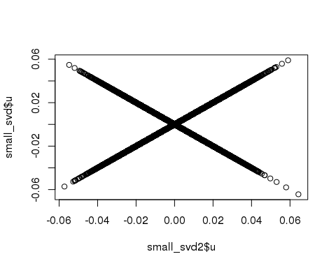
system.time(
  small_svd3 <- big_randomSVD(mat, big_scale(), ind.col = 1:2000)
)
## user system elapsed
## 0.368 0.000 0.368plot(small_svd3$u, small_svd$u)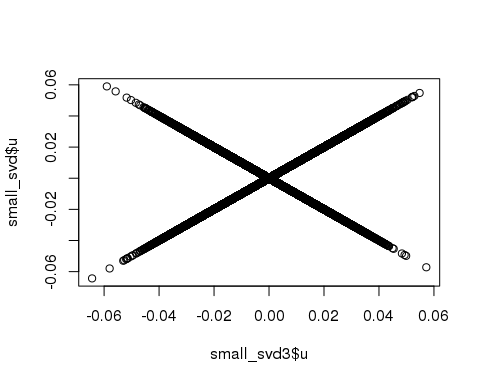
system.time(
  svd_all <- big_randomSVD(mat, big_scale())
)
## user system elapsed
## 1.810 0.056 1.862plot(svd_all)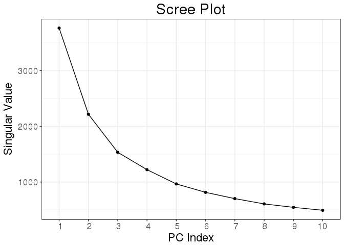
Function big_randomSVD() uses Rcpp and package Rpsectra to implement a fast Singular Value Decomposition for a FBM that is linear in all dimensions (standard PCA algorithm is quadratic in the smallest dimension) which makes it very fast even for large datasets (that have both dimensions that are large).
Some linear models
M <- 100 # number of causal variables
set <- sample(ncol(mat), M)
y <- mat[, set] %*% rnorm(M)
y <- y + rnorm(length(y), sd = 2 * sd(y))

ind.train <- sort(sample(nrow(mat), size = 0.8 * nrow(mat)))
ind.test <- setdiff(rows_along(mat), ind.train)

mult_test <- big_univLinReg(mat, y[ind.train], ind.train = ind.train,
covar.train = svd_all$u[ind.train, ])library(ggplot2)
plot(mult_test) +
aes(color = cols_along(mat) %in% set) +
labs(color = "Causal?")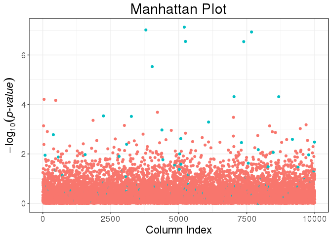
train <- big_spLinReg(mat, y[ind.train], ind.train = ind.train,
                      covar.train = svd_all$u[ind.train, ],
                      alpha = 0.5)
pred <- predict(train, X = mat, ind.row = ind.test, covar.row = svd_all$u[ind.test, ])
plot(apply(pred, 2, cor, y = y[ind.test]))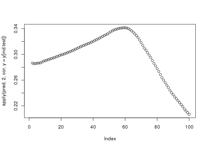
The functions big_spLinReg(), big_spLogReg() and big_spSVM() all use lasso (L1) or elastic-net (L1 & L2) regularizations in order to limit the number of predictors and to accelerate computations thanks to strong rules (R. Tibshirani et al. 2012). The implementation of these functions are based on modifications from packages sparseSVM and biglasso (Zeng and Breheny 2017). Yet, these models give predictions for a range of 100 different regularization parameters whereas we are only interested in one prediction.
So, that’s why I came up with the idea of Cross-Model Selection and Averaging (CMSA), which principle is:
- This function separates the training set in K folds (e.g. 10).
- In turn,
- each fold is considered as an inner validation set and the others (K - 1) folds form an inner training set,
- the model is trained on the inner training set and the corresponding predictions (scores) for the inner validation set are computed,
- the vector of scores which maximizes
fevalis determined, - the vector of coefficients corresponding to the previous vector of scores is chosen.
- The K resulting vectors of coefficients are then combined into one vector.
train2 <- big_CMSA(big_spLinReg, feval = function(pred, target) cor(pred, target),
                   X = mat, y.train = y[ind.train], ind.train = ind.train,
                      covar.train = svd_all$u[ind.train, ],
                      alpha = 0.5, ncores = nb_cores())
mean(train2 != 0) # percentage of predictors
## [1] 0.1285714pred2 <- predict(train2, X = mat, ind.row = ind.test, covar.row = svd_all$u[ind.test, ])
cor(pred2, y[ind.test])## [1] 0.3353398Some matrix computations
For example, let’s compute the correlation of the first 2000 columns.
system.time(
  corr <- cor(mat[, 1:2000])
)
## user system elapsed
## 11.015 0.006 11.018system.time(
corr2 <- big_cor(mat, ind.col = 1:2000)
)## user system elapsed
## 0.539 0.022 0.561class(corr2)## [1] "FBM"
## attr(,"package")
## [1] "bigstatsr"all.equal(corr2[], corr)## [1] TRUEAdvantages of using FBM objects
- you can apply algorithms on 100GB of data,
- you can easily parallelize your algorithms because the data on disk is shared,
- you write more efficient algorithms,
- you can use different types of data, for example, in my field, I’m storing my data with only 1 byte per element (rather than 8 bytes for a standard R matrix). See the documentation fo the FBM class for details.
In a next post, I’ll try to talk about good practices on how to use parallelism in R.
References
Kane, Michael J, John W Emerson, and Stephen Weston. 2013. “Scalable Strategies for Computing with Massive Data.” Journal of Statistical Software 55 (14): 1–19. doi:10.18637/jss.v055.i14.
Tibshirani, Robert, Jacob Bien, Jerome Friedman, Trevor Hastie, Noah Simon, Jonathan Taylor, and Ryan J Tibshirani. 2012. “Strong rules for discarding predictors in lasso-type problems.” Journal of the Royal Statistical Society. Series B, Statistical Methodology 74 (2): 245–66. doi:10.1111/j.1467-9868.2011.01004.x.
Wickham, Hadley. 2011. “The Split-Apply-Combine Strategy for Data Analysis. Journal of Statistical Software.” Journal of Statistical Software 40 (1): 1–29. doi:10.1039/np9971400083.
Zeng, Yaohui, and Patrick Breheny. 2017. “The biglasso Package: A Memory- and Computation-Efficient Solver for Lasso Model Fitting with Big Data in R,” January. http://arxiv.org/abs/1701.05936.