IPython Notebook Essentials

There are several approaches to setting up an IPython notebook environment. We suggest you use Anaconda, a free distribution designed for large-scale data processing, predictive analytics, and scientific computing. Alternatively, you can use Wakari, which is a web-based installation of Anaconda. Wakari has several levels of service, but the basic level is free and suitable for experimenting and learning.

You are now ready to run the notebook. First, we create a directory named my_notebooks to hold your notebooks and open a terminal window at this directory. Different operating systems perform different steps.

Microsoft Windows users need to perform the following steps:

Mac OS X and other Unix-like systems' users need to perform the following steps:

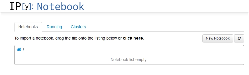
After a while, your browser will automatically load the notebook dashboard as shown in the following screenshot. The dashboard is a mini filesystem where you can manage your notebooks. The notebooks listed in the dashboard correspond exactly to the files you have in the directory where the notebook server was launched.

Creating a Wakari account

To access Wakari, simply go to https://www.wakari.io and create an account. After logging in, you will be automatically directed to an introduction to using the notebook interface in Wakari. This interface is shown in the following screenshot:

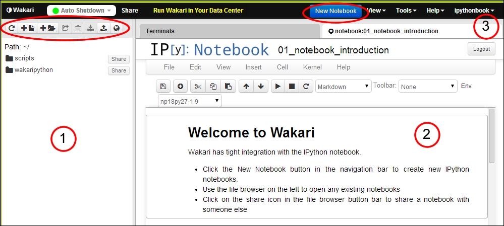
The interface elements as seen in the preceding screenshot are described as follows:

• The section marked 1 shows the directory listing of your notebooks and files. On the top of this area, there is a toolbar with buttons to create new files and directories as well as download and upload files.

• The section marked 2 shows the Welcome to Wakari notebook. This is the initial notebook with information about IPython and Wakari. The notebook interface is discussed in detail in Chapter 2, The Notebook Interface.

• The section marked 3 shows the Wakari toolbar. This has the New Notebook button and drop-down menus with other tools.

Note

This book concentrates on using IPython through the notebook interface. However, it's worth mentioning the two other ways to run IPython.

The simplest way to run IPython is to issue the ipython command in a terminal window. This starts a command-line session of IPython. As the reader may have guessed, this is the original interface for IPython.

Alternatively, IPython can be started using the ipython qtconsole command. This starts an IPython session attached to a QT window. QT is a popular multiplatform windowing system that is bundled with the Anaconda distribution. These alternatives may be useful in systems that, for some reason, do not support the notebook interface.

Creating your first notebook

We are ready to create our first notebook! Simply click on the New Notebook button to create a new notebook.

• In a local notebook installation, the New Notebook button appears in the upper-left corner of the dashboard.

• In Wakari, the New Notebook button is at the top of the dashboard, in a distinct color. Do not use the Add File button.

Notice that the Wakari dashboard contains a directory list on the left. You can use this to organize your notebooks in any convenient way you choose. Wakari actually provides access to a fully working Linux shell.

We are now ready to start computing. The notebook interface is displayed in the following screenshot:

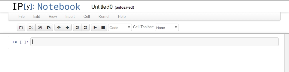
By default, new notebooks are named UntitledX, where X is a number. To change it, just click on the current title and edit the dialog that pops up.

At the top of the notebook, you will see an empty box with the In [ ]: text on the left-hand side. This box is called a code cell and it is where the IPython shell commands are entered. Usually, the first command we issue in a new notebook is %pylab inline. Go ahead and type this line in the code cell and then press Shift + Enter (this is the most usual way to execute commands. Simply pressing Enter will create a new line in the current cell.) Once executed, this command will issue a message as follows:

Populating the interactive namespace from numpy and matplotlib

This command makes several computational tools easily available and is the recommended way to use the IPython notebook for interactive computations. The inline directive tells IPython that we want graphics embedded in the notebook and not rendered with an external program.

Commands that start with % and %% are called magic commands and are used to set up configuration options and special features. The %pylab magic command imports a large collection of names into the IPython namespace. This command is usually frowned upon for causing namespace pollution. The recommended way to use libraries in scripts is to use the following command:

import numpy as np

Then, for example, to access the arange() function in the NumPy package, one uses np.arange(). The problem with this approach is that it becomes cumbersome to use common mathematical functions, such as sin(), cos(), and so on. These would have to be entered as np.sin(), np.cos(), and so on, which makes the notebook much less readable.

In this book, we adopt the following middle-of-the road convention: when doing interactive computations, we will use the %pylab directive to make it easier to type formulae. However, when using other libraries or writing scripts, we will use the recommended best practices to import libraries.

Suppose you get a cup of coffee at a coffee shop. Should you mix the cream into the coffee at the shop or wait until you reach your office? The goal, we assume, is to have the coffee as hot as possible. So, the main question is how the coffee is going to cool as you walk back to the office.

The difference between the two strategies of mixing cream is:

We need a model for the cooling process. The simplest such model is Newton's cooling law, which states that the rate of cooling is proportional to the temperature difference between the coffee in the cup and the ambient temperature. This reflects the intuitive notion that, for example, if the outside temperature is 40°F, the coffee cools faster than if it is 50°F. This assumption leads to a well-known formula for the way the temperature changes:

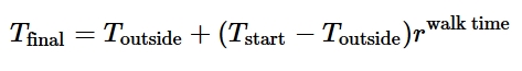
The constant r is a number between 0 and 1, representing the heat exchange between the coffee cup and the outside environment. This constant depends on several factors, and may be hard to estimate without experimentation. We just chose it somewhat arbitrarily in this first example.

We will start by setting variables to represent the outside temperature and the rate of cooling and defining a function that computes the temperatures as the liquid cools. Then, type the lines of code representing the cooling law in a single code cell. Press Enter or click on Return to add new lines to the cell.

As discussed, we will first define the variables to hold the outside temperature and the rate of cooling:

temp_out = 70.0
r = 0.9

After entering the preceding code on the cell, press Shift + Enter to execute the cell. Notice that after the cell is executed, a new cell is created.

Next, we define the function representing the cooling law:

def cooling_law(temp_start, walk_time):
    return temp_out + (temp_start - temp_out) * r ** walk_time 

The cooling_law()function accepts the starting temperature and walking time as the input and returns the final temperature of the coffee. Notice that we are only defining the function, so no output is produced. In our examples, we will always choose meaningful names for variables. To be consistent, we use the conventions in the Google style of coding for Python as shown in http://google-styleguide.googlecode.com/svn/trunk/pyguide.html#Python_Language_Rules.

TypeError: unsupported operand type(s) for ^: 'float' and 'float'

We can now compute the effect of cooling given any starting temperature and walking time. For example, to compute the temperature of the coffee after 10 minutes, assuming the initial temperature to be 185°F, run the following code in a cell:

cooling_law(185.0, 10.0)

The corresponding output is:

110.0980206115

What if we want to know what the final temperature for several walking times is? For example, suppose that we want to compute the final temperature every 5 minutes up to 20 minutes. This is where NumPy makes things easy:

times = arange(0.,21.,5.)
temperatures = cooling_law(185., times)
temperatures

We start by defining times to be a NumPy array, using the arange() function. This function takes three arguments: the starting value of the range, the ending value of the range, and the increment.

After defining the times array, we can simply call the cooling_law() function with times as the second argument. This computes the temperatures at the given times.

Once we have the temperatures, we can display them in a graph. To display the graph, execute the following command line in a cell:

plot(times, temperatures, 'o')

The preceding command line produces the following plot:

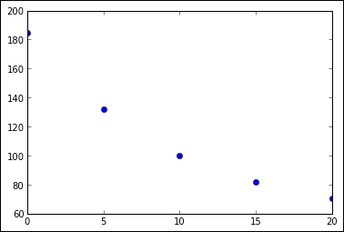
The plot() function is a part of the matplotlib package, which will be studied in detail in Chapter 3, Graphics with matplotlib. In this example, the first two arguments to plot() are NumPy arrays that specify the data for the horizontal and vertical axes, respectively. The third argument specifies the plot symbol to be a filled circle.

We are now ready to tackle the original problem: should we mix the cream in at the coffee shop or wait until we get back to the office? When we mix the cream, there is a sudden drop in temperature. The temperature of the mixture is the average of the temperature of the two liquids, weighted by volume. The following code defines a function to compute the resulting temperature in a mix:

def temp_mixture(t1, v1, t2, v2):
    return (t1 * v1 + t2 * v2) / (v1 + v2)

The arguments in the function are the temperature and volume of each liquid. Using this function, we can now compute the temperature evolution when the cream is added at the coffee shop:

temp_coffee = 185.
temp_cream = 40.
vol_coffee = 8.
vol_cream = 1.
initial_temp_mix_at_shop = temp_mixture(temp_coffee, vol_coffee, temp_cream, vol_cream)
temperatures_mix_at_shop = cooling_law(initial_temp_mix_at_shop, times)
temperatures_mix_at_shop

As usual, type all the commands in a single code cell and then press Shift + Enter to run the whole cell. We first set the initial temperatures and volumes for the coffee and the cream. Then, we call the temp_mixture() function to calculate the initial temperature of the mixture. Finally, we use the cooling_law() function to compute the temperatures for different walking times, storing the result in the temperatures_mix_at_shop variable. The preceding command lines produce the following output:

array([ 168.88888889,  128.3929    ,  104.48042352,   90.36034528,
         82.02258029])

Remember that the times array specifies times from 0 to 20 with intervals of 5 minutes. So, the preceding output gives the temperatures at these times, assuming that the cream was mixed in the shop.

To compute the temperatures when considering that the cream is mixed after walking back to our office, execute the following commands in the cell:

temperatures_unmixed_coffee = cooling_law(temp_coffee, times)
temperatures_mix_at_office = temp_mixture(temperatures_unmixed_coffee, vol_coffee, temp_cream, vol_cream)
temperatures_mix_at_office

We again use the cooling_law() function, but using the initial coffee temperature temp_coffee (without mixing the cream) as the first input variable. We store the results in the temperatures_unmixed_coffee variable.

To compute the effect of mixing the cream in after walking, we call the temp_mixture() function. Notice that the main difference in the two computations is the order in which the functions cooling_law() and temp_mixture() are called. The preceding command lines produce the following output:

array([ 168.88888889,  127.02786667,  102.30935165,   87.71331573,
         79.09450247])

Let's now plot the two temperature arrays. Execute the following command lines in a single cell:

plot(times, temperatures_mix_at_shop, 'o')
plot(times, temperatures_mix_at_office, 'D', color='r')

The first plot() function call is the same as before. The second is similar, but we want the plotting symbol to be a filled diamond, indicated by the argument 'D'. The color='r' option makes the markings red. This produces the following plot:

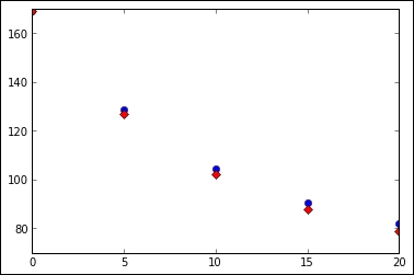
Notice that, by default, all graphs created in a single code cell will be drawn on the same set of axes. As a conclusion, we can see that, for the data parameters used in this example, mixing the cream at the coffee shop is always better no matter what the walking time is. The reader should feel free to change the parameters and observe what happens in different situations.

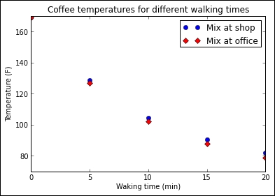
Scientific plots should make clear what is being represented, the variables being plotted, as well as the units being used. This can be nicely handled by adding annotations to the plot. It is fairly easy to add annotations in matplotlib, as shown in the following code:

plot(times, temperatures_mix_at_shop, 'o')
plot(times, temperatures_mix_at_office, 'D', color='r')
title('Coffee temperatures for different walking times')
xlabel('Waking time (min)')
ylabel('Temperature (F)')
legend(['Mix at shop', 'Mix at office']) 

After plotting the arrays again, we call the appropriate functions to add the title (title()), horizontal axis label (xlabel()), vertical axis label (ylabel()), and legend (legend()). The arguments to all this functions are strings or a list of strings as in the case of legend(). The following graph is what we get as an output for the preceding command lines:

There is something unsatisfactory about the way we conducted this analysis; our office, supposedly, is at a fixed distance from the coffee shop. The main factor in the situation is the outside temperature. Should we use different strategies during summer and winter? In order to investigate this, we start by defining a function that accepts as input both the cream temperature and outside temperature. The return value of the function is the difference of final temperatures when we get back to the office.

The function is defined as follows:

temp_coffee = 185.
vol_coffee = 8.
vol_cream = 1.
walk_time = 10.0
r = 0.9
def temperature_difference(temp_cream, temp_out):
    temp_start = temp_mixture(temp_coffee,vol_coffee,temp_cream,vol_cream)
    temp_mix_at_shop = temp_out + (temp_start - temp_out) * r ** walk_time
    temp_start = temp_coffee
    temp_unmixed =  temp_out + (temp_start - temp_out) * r ** walk_time
    temp_mix_at_office = temp_mixture(temp_unmixed, vol_coffee, temp_cream, vol_cream)
    return temp_mix_at_shop - temp_mix_at_office

In the preceding function, we first set the values of the variables that will be considered constant in the analysis, that is, the temperature of the coffee, the volumes of coffee and cream, the walking time, and the rate of cooling. Then, we defined the temperature_difference function using the same formulas we discussed previously. We can now use this function to compute a matrix with the temperature differences for several different values of the cream temperature and outside temperature:

cream_temperatures = arange(40.,51.,1.)
outside_temperatures = arange(35.,60.,1.)
cream_values, outside_values = meshgrid(cream_temperatures, outside_temperatures)
temperature_differences = temperature_difference(cream_values, outside_values)

The first two lines in the cell use the arange() function to define arrays that contain equally spaced values for the cream temperatures and outside temperatures. We then call the convenience function, meshgrid(). This function returns two arrays that are convenient to calculate data for three-dimensional graphs and are stored in the variables cream_values and outside_values. Finally, we call the temperature_difference() function, and store the return value in the temperature_differences array. This will be a two-dimensional array (that is, a matrix).

We are now ready to create a three dimensional plot of the temperature differences:

from mpl_toolkits.mplot3d import Axes3D
fig = figure()
fig.set_size_inches(7,5)
ax = fig.add_subplot(111, projection='3d')
ax.plot_surface(cream_values, outside_values, temperature_differences, rstride=1, cstride=1, cmap=cm.coolwarm, linewidth=0)
xlabel('Cream temperature')
ylabel('Outside temperature')
title('Temperature difference') 

In the preceding code segment, we started by importing the Axes3D class using the following line:

from mpl_toolkits.mplot3d import Axes3D

This class, located in the mpl_toolkits.mplot3d module, is not automatically loaded. So, it must be explicitly imported.

Then we create an object fig of the class figure, set its size, and generate an object ax that is an object of the class Axes3D. Finally, we call the ax.plot_surface() method to generate the plot. The last three command lines set the axis labels and the title.

The output of the preceding command lines will produce the following graph:

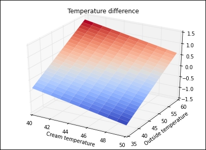
Notice the cmap=cm.coolwarm argument in the call to ax.plot_surface(). This sets the color map of the plot to cm.coolwarm. This color map conveniently uses a blue-red gradient for the function values. As a result, negative temperature differences are shown in blue and positive temperatures in red. Notice that there seems to be a straight line that defines where the temperature difference transitions from negative to positive. This actually corresponds to values where the outside temperature and the cream temperature are equal. It turns out that if the cream temperature is lower than the outside temperature, we should mix the cream into the coffee at the coffee shop. Otherwise, the cream should be poured in the office.

The following are some practice questions that will help you to understand and apply the concepts learned in this chapter:

In this chapter, we set up an IPython environment with Anaconda, accessed the IPython notebook online through Wakari, created a notebook, and learned the basics of editing and executing commands, and lastly, we went through an extensively applied example featuring the basic notebook capabilities.

In the next chapter, we will delve more deeply in the facilities provided by the notebook interface—including notebook navigation and editing facilities, interfacing with the operating system, loading and saving data, and running scripts.