Using BigQuery ML and BigQuery GIS together to predict NYC taxi trip cost

In this article, I’ll walk you through the process of building a machine learning model using BigQuery ML. As a bonus, we’ll have the chance to use BigQuery’s support for spatial functions.

We’ll use the New York City taxicab dataset, with the goal of predicting taxi fare, given both pick-up and drop-off locations for each ride — imagine that we are designing a trip planner.

Create a training dataset

The first step is to set up a machine learning dataset. In BigQuery, we simply write this query:

Note a few things about the query:

1. The main part of the query is at the bottom: (SELECT * from taxitrips)

2. taxitrips does the bulk of the extraction for the NYC dataset, with the SELECT containing my training features and label.

3. The WHERE removes data that I don’t want to train on.

4. The WHERE also includes a sampling clause to pick up only 1/1000th of the data

5. I define a variable called TRAIN so that I can quickly build an independent EVAL set. Note that BigQuery will automatically split the TRAIN data into two parts, and use one part of the training dataset to do things like early stopping and learning rate exploration. I am creating an independent evaluation dataset that I will not show to BigQuery during training.

Training the model

Once I have a query to create the training dataset, I can now train the model by prepending a few lines to the creation query:

Note a few things about the above query:

1. CREATE model is a safe way to ensure that you don’t overwrite existing models. CREATE or REPLACE will … replace existing models.

2. I specify my model type. Use linear_reg for regression problems and logistic_reg for classification problems.

3. I specify that the total_fare column is the label.

4. I ask that model training stop when the improvement is < 0.5% (this is optional, but shows you how to specify any optional parameters).

Running the query takes about 5 minutes on the 1-million row training dataset. Pause for a minute and take that in: it only takes 5 minutes to train an ML model on 1 million rows!

Evaluating the model

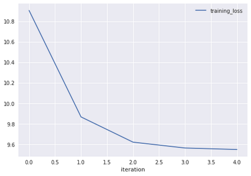
The training loss is not especially interesting, though. What we want is to evaluate the model on an independent dataset. We can do that by changing the TRAIN to EVAL in the training dataset query and computing the RMSE (root-mean-square error) as follows:

The important idea here is that you run ML.PREDICT to pass in the trained model, and then issue a select statement consisting of the rows on which you want to evaluate. Since my label is called ‘total_amount’, ML.PREDICT will provide me a ‘predicted_total_amount’. I can use that to compute the RMSE.

In this case, my model returns a RMSE of $9.57. Can we do better?

Faceted evaluation

We can write a more sophisticated evaluation that computes the mean absolute percent error (MAPE) and group it by the taxi fare to see how the error varies with amount:

Plotting the MAPE by the original amount gives us:

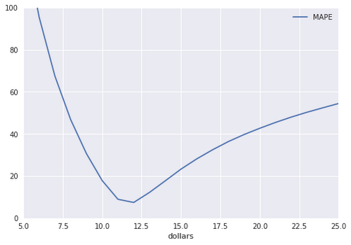
As you can see, we have serious problems, because  our error increases quadratically on either side of the mean.

I think we can do better.

Feature engineering with spatial and temporal features

Also, let’s allow the model to learn traffic patterns by creating a new feature that combines the time of day and day of week (this is called a feature cross). We can do that by:

CONCAT(dayofweek, CAST(hourofday AS STRING)) AS dayhr_fc

Finally, let’s feature cross the pick-up and drop-off locations so that the model can learn pick-up-drop-off pairs that will require tolls:

CONCAT(ST_AsText(ST_SnapToGrid(pickup, 0.1)),
       ST_AsText(ST_SnapToGrid(dropoff, 0.1))) AS loc_fc

This step takes the geographic point corresponding to the pickup point and grids to a 0.1-degree-latitude/longitude grid (approximately 8km x 11km in New York—we should experiment with finer resolution grids as well). Then, it concatenates the pickup and dropoff grid points to learn “corrections” beyond the Euclidean distance associated with pairs of pickup and dropoff locations.

Here’s the full query that runs all three of the above steps:

Notice also that I have greatly expanded the WHERE clause to limit the data to taxi-trips — data cleanup is very important!

The new model achieves a RMSE of $5.08, dropping the error by nearly 40%! Here is the training query and here is the evaluation query.

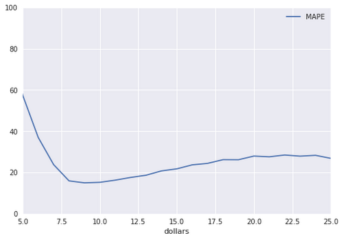
Mapping the evaluation results

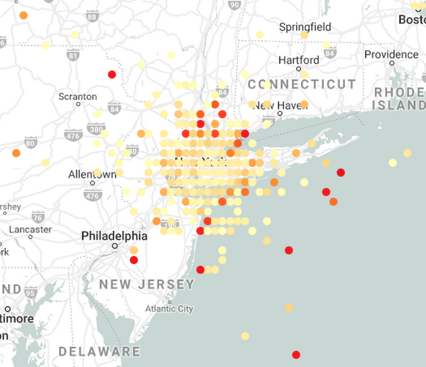
Instead of grouping by the total amount, we can group by a spatial feature. Let’s look at how the taxi fare error varies depending on the drop-off point:

Essentially, I am computing the mean absolute percent error by grouping based on the dropoff gridpoint. I then plotted it using the BigQuery Geo Viz (you will get a link to the tool when your project gets whitelisted):

Essentially, I am computing the mean absolute percent error by grouping based on the dropoff gridpoint. I then plotted it using the BigQuery Geo Viz (you will get a link to the tool when your project gets whitelisted):

Filtering on frequent drop-off areas and adjusting the color scale, we get:

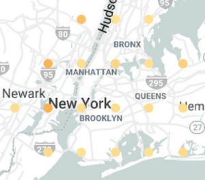
The larger errors correspond to out-of-town trips to Westchester and Jersey. It appears that such trips incur surcharges that the model hasn’t learned.

To learn more

1. Check out my notebook that includes full code on GitHub. (also includes full workflow, graphs, etc.)

2. The training query (uses CREATE MODEL)

3. The evaluation query (uses ML.EVALUATE)

4. The faceted evaluation (uses ML.PREDICT)

Enjoy!